This is third tutorial of our TRIVIAL SORTING ALGORITHMS series and before going further to another solution that introduce Insertion Sort, let us revisit the problem statement and constraints involved.
Problem Statement:
Suppose you have a microcontroller or embedded system, in which you need to implement a sorting mechanism. It takes an array and its size as input and sort the given array.
Constraints:
1. Code footprint should not be more than some KB.
2. Stack size is very limited so do not use any form of recursion.
3. Memory is limited so try to minimize the space complexity.
Sample Data Property:
In the practical scenario size of data is not more than 50 elements and also having minimum inversion or partially sorted.
Solution:
For the sake of simplicity we will construct our algorithms on integer array a[] containing N elements.
We have already stated that we would present a trivial sorting algorithm as one of the solution, as Merge sort, Quick sort and Heap sort have complex structures and each involve the recursion as an essential part to their solution. So in this third tutorial of our TRIVIAL-SORTING ALGORITHMS series we will analyze the Insertion Sort as one of the solution.
Just like the Selection Sort, in this approach also, we consider that the array consist of two sub lists one is sorted and resides at the left and another is unsorted and resides at the right. At the beginning, sorted list is empty and unsorted list consists of all the objects in the array.
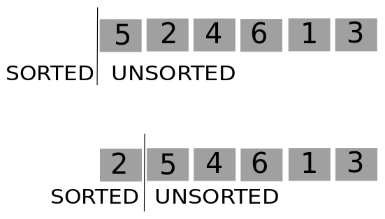
Insertion sort works in sorted list which is empty at first. It compare new element from unsorted list to the last element of sorted list and swap if necessary and move on to traverse the sorted list until it finds the element less than inserted element.
Following is the code snippet for insertion sort:
 for(int i=0;i<N;i++)
{
     for(int j=i;j>0;j--)
     {
        if(a[j] < a[j-1] )
        {
	   int tmp = a[j];
           a[j] = a[j-1];
	   a[j-1] = tmp;
        }
        else
        {
            break;
        }
     }
}
In the worst case where given array is reverse sorted, we still go through the array N^2 times making it bad for large number of elements, but given the property of data in the problem statement, this algorithm takes advantage of partially sorted array. Consider the following situation:
1, 5, 13, 20, 23, 32, 27
Here i= 27 and the sorted list will contain [1, 5, 13, 20, 23, 32]. So in this case N=7 and we will have only seven comparison and one swap as the array is partially sorted, making it more efficient than Bubble and selection sort. Now let us take this algorithm as base and enhance it further.
Consider the following situation:
3, 5, 13, 20, 23, 32, 1
According to current code following will be the stages:
3, 5, 13, 20, 23, 1, 32

3, 5, 13, 20, 1, 23, 32

3, 5, 13, 1, 20, 23, 32

3, 5, 1, 13, 20, 23, 32

3, 1, 5, 13, 20, 23, 32

1, 3, 5, 13, 20, 23, 32
Here the Bold elements represent where assignments have been done. We would have 3 assignments per swap making it 6*3= 18 assignments during the process.
As it is evident that 1 has to go to the first so we will not assign it to any index until we find the element less than 1. So observe the following changes in the code
for(int i=0;i<size;i++)
{
	int tmp = a[i];
	int j = i;
	for(j=i;j>0;j--)
	{
		if(tmp < a[j-1] )
		{
			a[j] = a[j-1];
		}
		else
		{
			break;  ---------------- (1)
		}
	}
	a[j] = tmp;
}
-
( Break is very important as it stop the comparison as soon as a smaller element is encountered.)
According to these changes stages are as follows:
tmp = 1
3, 5, 13, 20, 23, 32, 32

3, 5, 13, 20, 23, 23, 32

3, 5, 13, 20, 20, 23, 32

3, 5, 13, 13, 20, 23, 32

3, 5, 5, 13, 20, 23, 32

3, 3, 5, 13, 20, 23, 32

1, 3, 5, 13, 20, 23, 32
No we can see that number of assignments have been reduced to 7+2 (9) in comparison to 18. It is not much but in embedded environment even one assignment matter.
Now that we have enhanced the insertion sort, let us analyse its complexity.
1st passage through the for loop → 1 comparison and possible assignment.
2nd passage through the for loop → 2 comparison and possible assignment.
N - 1 passage through the for loop → N - 1 comparison and possible assignment.
if C is the constant time required for one comparison, one assignment, loop condition checking and increment of j then total time → C*( N - 1 + N - 2 + ... + 2 + 1 )
Let K be the total cost for assignment of tmp variable and N variable and checking condition of on i then → K(N - 1) as outer loop is executed for N - 1 time max
so final cost → C*( N (N - 1) /2 ) + K (N - 1) + K1 ~ O (N ^2)
K1 being some extra cost of initialization and other stuffs.
Now the extra space complexity is → c* 1 as only one extra variable last is used → O(1).
From this analysis it seems that insertion sort is no better than Bubble or selection sort in case of worst case. But given the property of the the Sample Data, we have partially sorted array with little number of inversion, thus leading to better performance of this algorithm.
Insertion sort propose the solution that most likely be used as the final solution, but in the next and final post of our TRIVIAL SORTING ALGORITHMS series, we will look in to the generic case of Insertion Sort also known as Shell Sort as our final and most viable solution.