In the last tutorial, we have witnessed the working of Quick Sort algorithm and also analysed the worst case of it. As promised, we will analyse the average case of Quick Sort and prove that it is in fact \(O(NlogN)\) as we had promised. But, before moving forward, let us formalise the claim we are making:

For every input array of length \(N\), Average running time of Quick Sort is \(O(NlogN)\) (by using the random pivots) .

As we have already stated that choosing a pivot is a crucial step in Quick Sort, we will form our proof around the Partitioning step. To avoid bad choices of pivots we either shuffle the array first and then choose the first element as a pivot or we choose a random pivot each time (both essentially have the same outcome).

At first, let's just check the best case. You must be wondering that why should we bother about the best case? In fact, we should never go for the Best case! But sometimes, if you want to check that how well your algorithm can do, you can find out using the Best Case analysis. So what would be the best case of Quick Sort or we should say Partition subroutine? Choose a pivot that partitions the array into two equal parts i.e. choose the median. We can not be that lucky to choose the median as a pivot in each recursive call but for the sake of argument let us just assume that we are, and that we chose the median as pivot in each recursive calls. In this situation, we can represent the running time of Quick Sort in a recurrence relation:

\(T(N) = 2T(N/2) + C*O(N)\)

We are recursing two times but for half of the input size and doing some linear amount of work in the Partition subroutine as the pivot gets compared with all the remaining elements once. We have seen this recurrence relation before in Merge Sort and know its solution to be \(O(NlogN)\) Now that we know how best Quick Sort can perform, one might suspect that the Average case would be costlier than the Best case! But in practice, it closely matches the Best case.

To prove this, we would be using some probability concepts namely sample space, random variables, expectation and linearity of expectation. We are assuming that you are familiar with these concepts.

Consider an array A of input size \(N\) :

Then, sample space \(\Omega\) = all possible outcomes of randomly picking a pivot in Quick Sort.

Let \(\sigma\) be the random variable for the pivot chosen such that \(\sigma \in \Omega \) and \(C(\sigma)\)= Number of comparisons between two elements made by Quick Sort (given random choices \(\sigma\))

Now since running time of Quick Sort is dominated by the comparisons, we would calculate the running time, as the average number of (or Expectation of) comparisons made by the algorithm. Thus, running time of Quick Sort = \(E[C]\) . Then, to prove our claim, we will have to prove that\(E[C] = O(NlogN)\).

Given that A = Input array with length N.

Let \(Z_i = \) i^th smallest element of Array A. It means that in an array \(A = 3, 6, 2, 1\) . 3 is 3^rd smallest and 6 is 4^th smallest element.

For ​\(\sigma \in \Omega \), ​\(X_{ij}(\sigma) = \) # of comparison between \(Z_i\) and \(Z_j\) in Quick Sort with Pivot sequence \(\sigma\)

At this moment, we want you to think about the number of times comparisons between \(Z_i\) and \(Z_j\) can happen in Quick Sort algorithm. In each Partition subroutine, every other element is compared with the Pivot element. So \(Z_i\) and \(Z_j\) can only be compared iff one of them is pivot and then, next comparison will not happen as the pivot is excluded in next recursive calls. So we would have either 0 or 1 comparison between \(Z_i\) and \(Z_j\) .

Now think about our first random variable \(C(\sigma)\) in terms of \(X_{ij}(\sigma)\) . We can express it as

\(C(\sigma) = \sum_{i=1}^{N-1} \sum_{j=i+1}^{N} X_{ij}(\sigma)\)

\(E[C] =E[ \sum_{i=1}^{N-1} \sum_{j=i+1}^{N} X_{ij} ]\)

Then, by linearity of Expectation we have \(E[C] = \sum_{i=1}^{N-1} \sum_{j=i+1}^{N} E[X_{ij}]\)

Since \(E[X_{ij}] = 0* p[X_{ij}=0] + 1* p[X_{ij}=1] = p[X_{ij}=1] \) i.e. probability of \(Z_i\) and \(Z_j\) get compared,

\(E[C] = \sum_{i=1}^{N-1} \sum_{j=i+1}^{N} p[X_{ij}=1]\)

Now we just have to find out the probability of \(Z_i\) and \(Z_j\) getting compared. For this, let's fix the \(Z_i\) and \(Z_j\) such that \(i < j\) and consider the set \(Z_i, Z_{i+1}, ..., Z_{j-1},Z_j\). As long as none of the elements of this set is chosen as the pivot, all are passed to the same recursive calls. Considering the first among \(Z_i, Z_{i+1}, ..., Z_{j-1},Z_j\) that gets chosen as pivot, then:

Case 1: if \(Z_i\) or \(Z_j\) gets chosen as Pivot then both get compared.

Case 2: if one of \(Z_{i+1}, ..., Z_{j-1}\) gets chosen as the pivot, then \(Z_i\) and \(Z_j\) are never compared as they are split between two recursive calls. So the sample space of Pivot choosing would be size of this set, i.e. \(j-1+1\) and favorable number of events would be 2 (either \(Z_i\) or \(Z_j\) got chosen as the pivot). This can be expressed as probability

\(p[X_{ij}=1] = \frac{2}{(j-i+1)}\)

thus \(E[C] = \sum_{i=1}^{N-1} \sum_{j=i+1}^{N} \frac{2}{(j-i+1)}\)

\(E[C] = 2* \sum_{i=1}^{N-1} \sum_{j=i+1}^{N}\frac{1}{(j-i+1)}\)

Now, if we can prove that the above equation is bounded by \(NlogN\), our claim will be validated. So let's find out how big this double summation term can be.

For each fixed value of i, the inner sum is \(\sum_{j=i+1}^{N} \frac{1}{(j-i+1)} = \frac{1}{2} + \frac{1}{3} + \frac{1}{4} + \dots\) and i can range from 1 to N-1

So \(E[C] <= 2* N*\sum_{k=2}^{N} \frac{1}{k}\)

Think of rectangles having width of 1 unit and height of \(\frac{1}{2} , \frac{1}{3}, \frac{1}{4} \dots\) and so on then the term \(\sum_{k=2}^{N} \frac{1}{k}\) will represent the sum of area of all such rectangles and it will be upper bounded by the area under the curve of \(\frac{1}{x}\) as shown in the diagram bellow.

(Image Source)

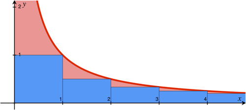
So \(\sum_{k=2}^{N} \frac{1}{k} <= \int_1^N \frac{1}{x} \: \mathrm{d}x\)

\(\sum_{k=2}^{N} \frac{1}{k} <= logN\)

so \(E[C] <= 2* N* logN = O(NlogN)\)

Thus, our claim that the average number of comparisons in Quick Sort is of the order \(O(NlogN)\) is proved. Please note that this tutorial is adapted from the coursera Video lectures of Tim Roughgarden. If you want more details or the video version you can consult coursera lectures.