In the second tutorial of our Divide and Conquer Algorithms series, we will analyse the Quick Sort algorithm. Before moving forward let us formalise the input/output of our algorithm.
INPUT: An array \(A[ ]\) containing \(N\) elements.
OUTPUT: A sorted array \(A[ ]\) containing \(N\) elements.
We have already discussed the Divide and Conquer approach, which gives us three stages of the algorithm i.e. Divide, Solve and Combine. So let us analyse the stages one by one in Quick Sort algorithm.
The first step would be to divide the problem into sub-problems, i.e. divide the input array into sub-arrays. In Merge Sort this step was trivial - just divide input array into two halves from mid element. However, in Quick Sort, this is the most crucial step as in this step we would try to find an element called 'pivot' and divide the input into two parts from the pivot position.
So what is pivot? In lay terms, pivot is a point where a rotational system is pinned down. So, the whole system may move around, but pivot point stays at the same place. The analogy is almost exact here too.
Pivot is an element which is in the exact position after the array is sorted.
Pivot is an element which is in the exact position after the array is sorted. This means that all the elements lower than the pivot are to its left and all the elements higher than pivot are to its right.
Basic Idea for the pivot is to partition the array such that, for some index j as the pivot
- entry a[j] is in place.
- no larger entry is to the left of j.
- no smaller entry is to the right of j.
Sort each piece recursively.
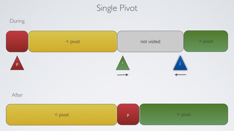
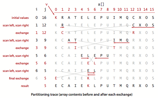
In practice, we can choose any element as pivot for partitioning. For simplicity let us just take the first element as pivot. So, an implementation for partitioning (choose first element as pivot) may look like:
lo = First element of array; %Short for Lower
i=lo+1;
j=hi; %short for Higher
Phase 1: Repeat until i and j cross.
- scan i left to right as long as (a[i]<a[lo]).
- scan j from right to left as long as (a[j] > a[lo]).
- exchange a[i] and a[j].
Phase 2: When the i and j cross.
1. exchange a[lo] and a[j].
int partition(int* a,int low, int hi)
{
	int i = low;
	int j = hi+1;

	int p = a[low];
	while(true)
	{
		while( a[++i] < p )
			if(i == hi) break;
		while( a[--j] > p)
			if(i == low) break;

		if(i >= j) break;

		int tmp = a[i];
		a[i] = a[j];
		a[j] = tmp;
	}
	a[low] = a[j];
	a[j] = p;
	return j;
}
The second stage of the algorithm would be to solve the subproblems. As stated in the Merge Sort tutorial, we form our base case when there is only one element left in the array. There is not much to do here as we would partition the array until there is only one element left in the subarray and when we reached that phase, the subproblem is solved.
Now the third step should be The Combine Step. In Merge Sort, this step was crucial as individual problems were sorted individually but overall they were largely unsorted. So we needed a mechanism to put them together in sorted order. But in the quick sort algorithm there is no need for this. Notice that in the partioning step, we find an element and put it in it's proper position. So, by the time we are through with the partition step and reach our combining case, we need not do anything as all the elements have been placed in their respective position and are where they should be in sorted array.
For completeness, the following is one implementation:
void quick_sort(int *a, int low, int hi)
{
	if(low >= hi)
		return;
	int p = partition(a,low,hi);
	quick_sort(a, low, p-1);
	quick_sort(a, p+1, hi);
}
Worst Case:
We have already seen that the most crucial step of this algorithm is choosing a pivot. So, if we want to think about the worst case we should focus on choosing the pivot such that the partition is unbalanced. As we are taking the first element as pivot and for this case assume that the array is reverse sorted, what might happen?
In this case, we would have to move all the elements to the left side of pivot as it is the largest element in the array. Let us take an example:
N = 10
PIVOT = 10
10 9 8 7 6 5 4 3 2 1
Iterator \(i\) points to \(9\) and \(j \) points to \(1\)
Now \(i\)will move forward and compare all the elements with pivot until we reach the end of array leading to \(N-1\) comparisons. Now \(j\) will move backward but will encounter a smaller element than the pivot and will stop, leads to \(1\) comparison.
So in one partition routine, we will have \(N\) comparisons for input size \(N\) .
After this step, one array would contain 9 elements and another array would be empty. Now this N - 1 element array will also take N - 1 compare and switching. If we sum it up it leads to
\(N + N-1 + N-2 + ... + 3 + 2 + 1 = N(N+1)/2\)
So Number of comparisons is of quadratic order ~ \(1/2*N^2\)
Average case:
On an average Quick Sort complexity is \(O(NlogN)\) and in fact, it takes 39% more comparisons than Merge Sort. But, it is faster than Merge Sort in practice because of less data movement. So, how to avoid the worst case? use random shuffle (we will talk about the average case more in the another tutorial)
Improvements:
- Cutoff at 10 by insertion sort.
- Best choice of pivot item is median.
Estimate the true median by taking samples of 3 random items.
Practical usage:
1. Java uses it for sorting the primitive types.
2. C qsort, Unix, Visual C++, Python, Matlab, chrome JavaScript.
In this tutorial, we have explained the Quick Sort steps and implementation and we also talked about the worst case of the algorithm, but still we owe you some explanation about the average time being \(O(NlogN)\). So in the next tutorial, we will talk about the average case analysis of Quick Sort Algorithm and prove that it is in fact \(O(NlogN)\).