In this tutorial, we will implement the Heap Data Structure from scratch and see how we can perform various operations with the desired running time complexity.
\r\n\r\nIn the previous tutorial, we described how Heaps can be used for choosing minimum/maximum item in each iteration and also promised an explanation of their inner workings due to which we can achieve the performance stated before. Before moving forward let's see the definition of Heap from Wikipedia once again:
\r\n\r\n\r\n\r\n\r\nIn computer science, a heap is a specialized tree-based data structure that satisfies the heap property: If A is a parent node of B then the key of node A is ordered with respect to the key of node B with the same ordering applying across the heap. A heap can be classified further as either a "max heap" or a "min heap".
\r\n
It states that the Heap is a tree-based data structure and in practice, it is implemented as a Complete Binary Tree. If the complete binary tree follows the heap property stated above then we call it a Heap. Consider following two statements:
\r\n\r\n\r\n\r\n\r\n\r\n\t
\r\n\r\n- A binary tree is full if each node is either a leaf or possesses exactly two child nodes.
\r\n\r\n\r\n\r\n\t
\r\n- A binary tree is complete if all levels except possibly the last are completely full, and the last level has all its nodes to the left side.
\r\n
Following Diagram should clarify the distinction between a complete and a full binary tree:
\r\n\r\n
Now a Complete Binary tree can be implemented using most simple inbuilt data structure i.e. Array. The illustration below shows a complete binary tree representation in Array:
\r\n\r\n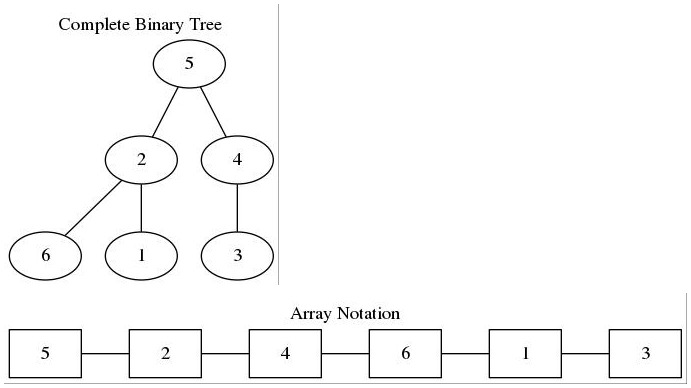
In the illustration above, we can see that node at index (i) has the parent at \\(\\lfloor {(i-1)/2}\\rfloor\\) (floor value), the left child is at \\(2*i +1\\) and the right child at \\(2*i + 2\\) (following 0 based index). So, for element 4 located at index 2, the parent is at 0 (element 5), the left child at index 5 (element 3).
\r\n\r\nSo now we know how to represent the Heap in the form of an Array; the only thing left is that it should follow the Heap property. For example, if we take the case of Min-Heap, then every parent must have key less than its children. Now we will create the Min-Heap from the set of elements taken from an Array while ensuring that the Heap property is intact and in the process we formulate our first utility function 'insertElement'. First, let's take an example:
\r\n\r\nLet the Input Array from where elements would be taken one by one is \\(A[6] = [5,2,4,3,1,6]\\). Initially, the Min Heap would be empty with capacity 6 \\(H[6] = [-,-,-,-,-,-]\\). For insertion of elements, the following conditions must hold:
\r\n\r\n- \r\n\t
- It must remain a Complete Binary Tree. (For this we need to insert new node in the last array index) \r\n\t
- It must retain the heap property. (If property is violated, we should swap the child and parent) \r\n
While maintaining above two invariants, the following illustration shows changes in heap:
\r\n\r\n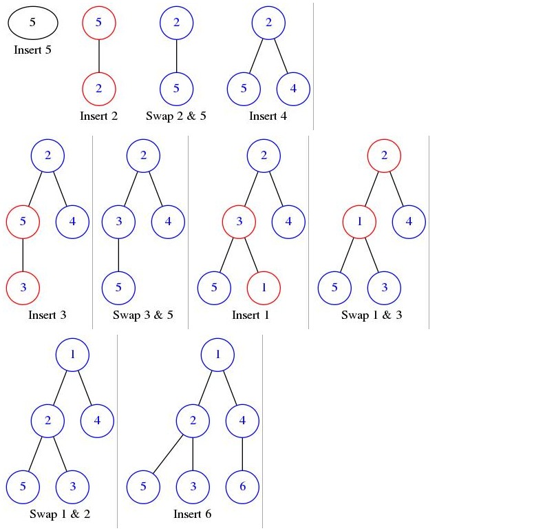
As evident from the illustration, insertion of element 2 violates the heap property and in order to restore it we need to swap the elements 2 and 5; same is the case with the insertion of element 3 (violations are marked with red circles). We can see that in the case of insertion of element 1, it takes two swaps before the heap property is restored. The procedure of exchanging child and parent node until the heap property is restored is formally called BubbleUp. So in our first utility function insertElement we will just insert the element at first available array index and then decide if we want to apply the BubbleUp operation or not based on the parent key. Following is the functional code:
\r\nvoid MinHeap::bubbleUp(int index)\r\n{\r\n\twhile(index != 0 && heap[parent(index)] > heap[index])\r\n\t{\r\n\t\tswap(&heap[parent(index)],&heap[index]);\r\n\t\tindex = parent(index); //----------------------------- (1)\r\n\t}\r\n}\r\n\r\nvoid MinHeap::insertElement(int key) {\r\n\tif(heap_size == capacity)\r\n\t{\r\n\t\tcout<<"Capacity full\\n";\r\n\t\treturn;\r\n\t}\r\n\theap_size++;\r\n\theap[heap_size -1] = key;\r\n\tbubbleUp(heap_size -1);\r\n}\r\n\r\nNow that we have a working code of insertElement, let us analyze the performance of this code and find out whether we fulfilled the expectations raised in our previous tutorial. These were the computational complexities that we claimed to achieve:
- \r\n\t
- Insertion - insert an element with cost \\(O (\\log N)\\) \r\n\t
- Deletion - delete an element at given index with cost \\(O (\\log N)\\) \r\n\t
- extractMin - Delete minimum key element with cost \\(O (\\log N)\\) \r\n\t
- getMin - get the minimum key element with cost \\(O(1)\\) \r\n\t
- InsertBulk - insert \\(N \\) elements in bulk with cost \\(O (N)\\) \r\n
The main work is done in the while loop of the BubbleUp function and it ends when Index is 0 or the parent has a lower key than its child. In the worst case, we say that the loop will end when Index reaches 0. Now if look at the line marked as (1), we realize that index is decreasing at the rate of \\((i-1)/2\\). So if we started at length \\(n\\) at worst case we will travel \\(\\log_2 n\\). It is easily seen if we try to write n in the nearest powers of two and argue that each division by 2 takes one exponent away. This way \\(\\log_{2}n = \\log_{2}2^h = h\\). This is exactly what we promised previously.
Min-Heap property states that each parent will have its key value lower than that of its children. So if the tree is fully heapified then the Minumum Key will always be at the root!; thus, function getMin have complexity in order of \\(O(1)\\) as we can access the first element of Array in constant time.
What about the extractMin and Deletion function? In fact extractMin is a Special case of Deletion in which the index value passed in 0. We'll understand deletion via an example, but before that let us first reiterate the invariants of delete operation and note some salient points:
- \r\n\t
- It must remain a Complete Binary Tree. Deletion is somewhat tricky; there is a difference between removing the Value in a node and removing the node itself. Here, we can't remove any random node as it will break the tree and that is not what we want. So what we will do is that we remove the value of given Node; copy the value of the last Node of the Heap to the given Node and then delete the last Node. In this way, the Heap will remain the Complete Binary tree. \r\n\t
- It must retain the heap property. In order to maintain the first invariant we have violated the second, so we must swap the child and parent until the property restored. \r\n
Following diagram shows working of extractMin on the Heap that we formed in the insertion step above:
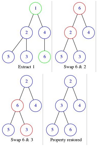
It should be evident from the illustration above that in one extractMin operation, we are traversing the tree the same number of times as is its height. This means we are traversing it \\(\\log_2 n\\) for n elements in the array; same time complexity is can be seen from the working code as follows:
\r\nvoid MinHeap::bubbleDown(int index)\r\n{\r\n\tint l = left(index);\r\n\tint r = right(index);\r\n\tint smallest = index;\r\n\r\n\tif(l < heap_size && heap[l] < heap[index])\r\n\t{\r\n\t\tsmallest = l;\r\n\t}\r\n\r\n\tif(r < heap_size && heap[r] < heap[smallest])\r\n\t{\r\n\t\tsmallest = r;\r\n\t}\r\n\r\n\tif(smallest != index)\r\n\t{\r\n\t\tswap(&heap[index],&heap[smallest]);\r\n\t\tbubbleDown(smallest);\r\n\t}\r\n}\r\n\r\nint MinHeap::extractMin() {\r\n\tif(heap_size == 0)\r\n\t\treturn 0;\r\n\telse if(heap_size == 1)\r\n\t{\r\n\t\theap_size--;\r\n\t\treturn heap[0];\r\n\t}\r\n\r\n\r\n\tint data = heap[0];\r\n\theap[0] = heap[heap_size-1];\r\n\theap_size--;\r\n\tbubbleDown(0);\r\n\treturn data;\r\n}\r\n\r\nIn the BubbleDown function, recursion happens for the smallest element and that is calculated as smallest of the two children of the current element. Since Index is increasing at the rate of \\(2*i\\) , for n elements we will reach the end after \\(\\log_2 n\\) iterations.
We have seen that the individual element insertion takes \\(\\log_2 n\\) time. This is pretty good in case of dynamic element insertion but still a heavy price if we are performing this operation for each of the elements we have in our static array; this is where bulkInsert plays its role. The idea is that we copy all the elements from the source Array to the Heap. In this way we are satisfying the first invariant that it should be a Complete Binary Tree, now all we need to do is to restore the heap property. Heap property can be restored via running bubbleDown on each of the parents from bottom to the top. But how will this operation restore the heap property? bubbleDown called with an Index ensures that a node at given index is at the right position with respect to its children and follow the heap property provided all of its children follow the same, so if we call bubbleDown for all the parents from bottom to top, then the whole tree will be heapify. For visual clarification, look at the example:
Let us say that heap has following elements after copying- \\(H[6] = [5,2,4,6,1,3]\\) . Following diagram shows the sequence of operations:
\r\n\r\n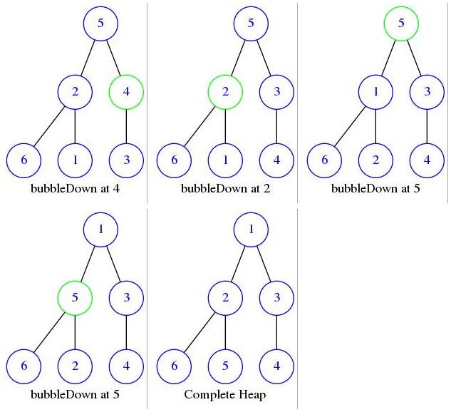
Now let's see the working code and analyze its running time complexity:
\r\n\r\n\r\nvoid MinHeap::bulkInsert(int* a,int size)\r\n{\r\n\tmemcpy(heap,a,size); //-------------------------------------(1)\r\n\theap_size = size;\r\n\tfor(int i = parent(heap_size-1);i >= 0; i--) //--------------(2)\r\n\t{\r\n\t\tbubbleDown(i);\r\n\t}\r\n}\r\n\r\nAt point (1), we are copying the elements from the given array. So if it has \\(n\\) elements then our running time complexity can't be less than \\(O(n)\\). Now, Time Complexity would be governed by processing of for loop. It is evident that we start at index \\(n/2\\) and go up to 0. We can say that the bubbleDown method is called \\(n/2\\) times and time complexity of bubbleDown method is \\(log_2 n\\) so the total time complexity should be \\(O(n\\text{ }log_2 n)\\). But in the earlier tutorial, we claimed the time complexity of \\(O(n)\\) for bulkInsert operation and indeed its average time complexity is \\(O(n)\\) . So, where we did we go wrong in our assessment? bubbleDown method has worst case time complexity of \\(log_2n\\) if it's called with Index 0. But in bulkInsert function bubbleDown for Index 0 is called only once and for all other nodes the depth up to which the element can descend is different. Following is the exact assessment of bubbleDown method for all the levels of Heap [1]:
Let's say that our tree is a complete tree that is \\(n = 2^{h+1} -1\\) where \\(h \\geq 0\\) is the height of Tree and its bottommost level is full. Now let's analyze the amount of work done for each level:
\r\n\r\n- \r\n\t
- (Bottom level 0) It will have \\(2^h\\) nodes and all of the nodes are Leaf so we don't call bubbleDown. \r\n\t
- (Bottom level 1) It will have \\(2^{h-1}\\) nodes and each of them can go down by 1 level. \r\n\t
- (Bottom level 1) It will have \\(2^{h-2}\\) nodes and each of them can go down by 2 level. \r\n\t
- (Bottom level i) It will have \\(2^{h-i}\\) nodes and each of them can go down by i level. \r\n
so calculating level by level, the Time complexity will be proportional to \\(T(n) = \\displaystyle\\sum_{i=0}^{h} Nodes_i * bubbleDown_i = \\sum_{i=0}^{h} 2^{h-i} * i\\) .
\r\n\r\nfactor \\(2^h\\) outside the summation :
\r\n\r\n\\( \\begin{equation} T(n) = \\displaystyle 2^h \\sum_{i=0}^{h} \\frac {i}{2^i} \\end{equation} \\) - (1)
\r\n\r\nNote that the equation (1) resembles an Arithmetico-geometric Progression. To solve equation (1) let us consider the sum of elements of a geometric series in which \\(r < 1\\) is given by
\r\n\r\n\\(\\displaystyle \\sum_{i=0}^{\\infty} r^i = \\frac {1} {1-r}\\)
\r\n\r\nNow Differentiate this equation with respect to r and multiply the result with r we get:
\r\n\r\n\\(\\displaystyle \\sum_{i=0}^{\\infty} i*r^{i-1} = \\frac {1} {(1-r)^2}\\)
\r\n\r\n\\(\\begin{equation} \\displaystyle \\sum_{i=0}^{\\infty} i*r^{i} = \\frac {r} {(1-r)^2} \\end{equation}\\) - (2)
\r\n\r\nNow if look at equation (1) and (2) closely we can achieve the similar formula as in summation part of equation (1) via equation (2) by putting the value of \\(r = 1/2\\). The difference will be that ours is a sum up to h while (2) goes on till infinity.
\r\n\r\n\\(\\displaystyle \\sum_{i=0}^{\\infty} \\frac{i}{2^i} = \\frac {1/2} {(1-1/2)^2} = \\frac{4}{2} = 2\\)
\r\n\r\nWe note that (2) will have more positive terms in summation and yet, it converges to a finite value of 2. This is the highest that we can get and will always be smaller than or equal to 2. In more technical parlance summation in equation (1) is finite bound, while summation in equation (2) is not bounded but still gives us the upper bound of 2. So we can say that:
\r\n\r\n\\(T(n) = \\displaystyle 2^h \\sum_{i=0}^{h} \\frac {i}{2^i} \\leq2^{h+1}\\)
\r\n\r\nNow according to our assumption \\(n = 2^{h+1} -1\\) i.e. \\(2^{h+1} = n +1\\) so
\r\n\r\n\\(T(n) = \\leq n+1 \\in O(N)\\)
\r\n\r\nWith this proof, we wrap up our discussion of Heap implementation. So in this post, we implemented insertElement, extractMin, getMin and bulkInsert for a data structure Min Heap and also analyzed their running time complexity. All these methods can be changed easily if you want to implement the Max Heap.