This is the second tutorial of our 'TRIVIAL SORTING ALGORITHMS' series and before going further to another solution that introduces Selection Sort, let us revisit the problem statement and constraints involved:
Problem Statement
Suppose you have a microcontroller or an embedded system, in which you need to implement a sorting mechanism. It takes an array and its size as input and sorts the given array.
Constraints:
- Code footprint should not be more than some kilobytes.
- Stack size is very limited so do not use any form of recursion.
- Memory is limited so try to minimize the space complexity.
Sample Data Property:
In a practical scenario, the size of data is not more than 50 elements at a time. Further, it also has minimum inversion; simply put, the incoming data is partially sorted.
Solution:
For the sake of simplicity, we will construct our algorithms on an integer array a[] containing N elements.
As we have already stated that we would present a trivial sorting algorithm as one of the solutions because Merge sort, Quick sort and Heap sort have complex structures and each involve recursion as an essential part to their solution. So in this second tutorial we will analyze the Selection Sort as one of the solutions.
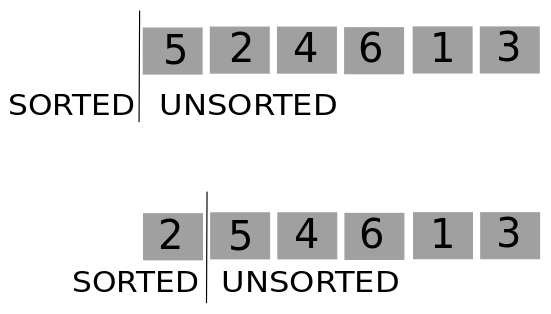
In this approach, we consider that the array consists of two sub-lists - one is sorted and resides at the left and the other is unsorted and is towards the right side. In the beginning, the sorted list is empty and unsorted list consists of all the objects in the array. The situation is depicted in the first figure shown below.
Selection Sort
In this algorithm, we define a rule first. We will partition the given array into two sets. The rule mandates that the set on the left will contain elements contained in a sorted order such that we cannot touch the element once we have put it there. Thus, no reordering of things in the left side. The right side contains the initial list. Initially, the left set is empty and the right set contains all the elements. As the algorithm proceeds, it keeps on putting one element per iteration from the left into the right. At any point in time, the algorithm is aware of how many elements it has put in the left set; this enables it to know at what index to put the next element. The situation is depicted graphically below.
Let us see the code for a basic algorithm and we will move to analyse its complexity and look for possible enhancements.
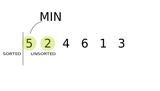
int i, iMin,j;

for(i=0;i<n-1;i++)
{
	iMin = i;
	for (j=i+1;j<n ;j++)
	{
              if(a[j] < a[iMin])
                    iMin = j;
	}

	if(i != iMin)
	{
		swap(a[iMin], a[i]);
	}
}
Consider the sequence:
Selection Sort
|6, 2, 4, 3, 9  → 2, |6, 4, 3, 9

2, |6, 4, 3, 9  → 2, 3, |4, 6, 9 // array is sorted but we have no way to recognize it

2, 3, |4, 6, 9   →  2, 3, 4, |6, 9 // No swap as i == iMin = 2 → a[i] = 4

2, 3, 4, |6, 9  →  2, 3, 4, 6, |9 // No swap as i == iMin = 3 → a[i] = 6
Here elements beyond the '|' sign indicate values that are present in the unsorted array (for loop in j) in which we have to find the minimum value. Upon analyzing this piece of code, we find that the algorithm does not make unnecessary swaps until it finds the minimum value in the right set. However, it is clear that we can not be certain that array is sorted or not just by checking the minimum values. That is, we have not been able to exploit the fact that the input data has minimum inversion! We unnecessarily looped at least thrice in this example. On this account, Selection sort is somewhat slower than Bubble sort when the array is partially sorted or have a little number of inversions.
Analysis:
1st passage through the for loop → N - 1 comparison and one possible swap.
2nd passage through the for loop → N - 2 comparison and possible swaps.
N - 1 passage through the for loop → 1 comparison and possible swaps.
if \(C\) is the constant time required for one comparison, one assignment, loop condition checking and increment of j then total time → \(C*[(N-1) + (N-2) + ... + 2 + 1]\)
Let \(K\) be the total cost for swap, assignment and checking condition on i. Then cost is \(K(N-1)\) as outer loop is executed \(N-1\) times at the maximum.
Therefore, the final cost is \(C \frac{N(N-1)}{2} + K(N-1) + K_1 \approx O (N^2)\) , \(K_1\) being some extra cost of initialization and other stuff.
Now the extra space complexity is \(C\) as only one extra variable iMin is used \(O(1)\)
As you can see that this algorithm takes time in multiples of N for finding the minimum value (inner loop ) and does it N times, leading to a worst case complexity to \(O(N^2)\). If we could somehow find an efficient way of finding Minimum Value, we would be able to improve this algorithm. Heap Sort implements this changes and finds the minimum value from the array in \(log(N)\) time thus reducing overall time complexity to \(O(NlogN)\) . We will study the Heap sort in later posts.
This post introduced you the Selection sort as one of the solutions of our problem, in the next post we will analyse Insertion Sort as one of our probable solutions.