In this post, we will see how we can accomplish the function done by Drag and Drop from the GUI by working directly on the underlying code itself. This post builds on the previous post of creating and visualizing time domain signals in GNU Radio.

So, the real meat of GNU Radio is in the python scripts. GNU Radio is all Python and C++. Here, we'll look into the python script autogenerated by GNU Radio Companion for us and start tinkering with it. First, let's have a look at the script and as we go, understand how flowgraphs are created in code as opposed to the drag and drop we did in the last post. The full script can be seen here.

class sinusoids(grc_wxgui.top_block_gui):

    def __init__(self):
        grc_wxgui.top_block_gui.__init__(self, title="Sinusoids")
        ...

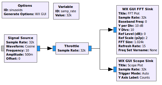
As we had said, the name we give to our flowgraph in ID acts as a master-class for our flow (class sinusoids). In its constructor, we instantiate various blocks that we want to use in our flowgraph and also set the sample rate that was named samp_rate. We have used 4 blocks: Signal Source, Throttle, FFT Sink and Oscilloscope Sink.

        self.wxgui_scopesink2_0 = scopesink2.scope_sink_c(
        	self.GetWin(),
        	title='Scope Plot',
        	sample_rate=samp_rate,
                ...
        )
        self.Add(self.wxgui_scopesink2_0.win)

The first statement creates an instance of the WX GUI Oscilloscope Sink with various parameters. The self.Add() method adds the instance to the flowgraph. Similarly, for FFT Sink Block. The instantiation and addition of GUI elements are done this way.

Other blocks do not usually require the Add method. Simple instantiation does it:

        self.blocks_throttle_0 = blocks.throttle(gr.sizeof_gr_complex*1, samp_rate,True)
        self.analog_sig_source_x_0 = analog.sig_source_c(samp_rate, analog.GR_COS_WAVE, 10, 0.5, 0)

The first statement initializes the throttle block while the second one initializes the signal source block with parameters (sample rate, cosine waveform, desired frequency, the amplitude of the signal and a phase offset).

A couple of interesting things: In the instantiation of the throttle block, the type of input expected is passed in as a parameter as gr.sizeof_gr_complex*1. In the case of a signal source, the module analog has two different methods sig_source_c and sig_source_f for complex and float type inputs respectively. As a rule, all the interconnections must have the same data types. That is - if one end of the connection has a data type complex, the other end must also accept complex data only (and not float).

Finally, we connect each block. This is simply by taking each pair of blocks and issuing the connect command:

        self.connect((self.analog_sig_source_x_0, 0), (self.blocks_throttle_0, 0))

This translates to - Connect analog source block's output Port Number 0 to throttle block's input Port Number 0.

There are a couple of other methods, and finally, we have the main execution block which instantiates our master class:

def main(top_block_cls=sinusoids, options=None):
    tb = top_block_cls()
    tb.Start(True)
    tb.Wait()

The Start() method starts execution and Wait() method makes the program run until there is some thread of the process still executing. Once we get a hang of these things, we can build more complex flowgraphs. The underlying mechanism is the same. These are directed graphs and data samples flow in the direction of the arrow.

The code for this python script is available on github. It creates the same flowgraph that we worked on in the previous post.

With this groundwork, we will start to tinker with it. What we would like to do now is create a signal in the frequency domain itself. For this, we will have to leave the safe harbour of GNU Radio Companion and start working on creating our own lightweight blocks for use. We see this in the next post.